Madison Math Circle: Mathematics of epidemics

Last night I had an amazing time at Madison Math Circle, hanging out with a bunch of bright school kids, who were undaunted by either diseases or mathematics. Since I had quite a few questions after the lecture, I decided to post an overview so anyone interested can go over it themselves. For those of you who attended and have further questions, or even wish to explore mathematical dynamics on your own, feel free to leave a comment below or e-mail me at marko@math.wisc.edu and I’ll try to answer all your questions and provide some guidance for future.

Today’s presentation was a glimpse into the world of applied math. Specifically, we discussed how mathematics can be used in messy context to give us estimates of phenomena for which we cannot build laboratory experiments: spread of epidemics. I have sprinkled a few questions around this explanation. If you have a calculation that answers them, write it out on a piece of paper, take a photo with a phone, and e-mail it to me at marko@math.wisc.edu . I’ll be very glad to hear from you and to discuss your calculations! The applets that I built can be freely modified by you using Sage/Python language. You can edit the code underneath the image to change the behavior of the applet. To start on your own, here’s an excellent website about using Sage in schools. And here is a free textbook covering college mathematics… but you’ll be able to work through some basics.

First, we talked about Daniel Bernoulli and how he worked out that variolation (immunization against smallpox by a small-scale infection) would save more lives than it would endanger, resulting in the increase of the mean life-time in the population. Open this PDF for a more detailed account of Bernoulli’s calculations. You can read about Bernoulli in general on this link.

Model is a set of equations or procedures that capture some quality of a natural process, e.g., a disease. We discussed compartmental models for a disease. Remember, instead of noting if a particular individual was infected or not, these models just count the proportion of healthy and proportion of sick people in the population. The same PDF as before has more on compartmental models.

Compartment model of a headache

The first model that we studied was a model for headache. We used $A[t]$ and $H[t]$ to denote the number of people who were Achin’ and Healthy in hour $t$ .

$\displaystyle A[t+1] = A[t] - g A[t] \\ H[t+1] = H[t] + g A[t]$
The constant $g$ is our get-well rate – the proportion of people that get well every hour. If you click on the image below, it will take you to the interactive applet we used in class.

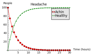
Click to go to the Sage applet for the headache model.

Notice that the time that it takes for half of the initial patients to get better, e.g., from 100 to 50 patients, or from 60 to 30, is always the same, no matter how many patients we start with. If we denote this time, called half life, by $t_H$ , the following equation says that at time $t_H$ the number of patients is exactly the half of the original number

$A[t_H] = \frac{1}{2} A[0]$ .

But what is that number? The equation $A[t+1] = A[t] - gA[t]$ can be rewritten as $A[t+1] = (1-g) A[t]$ which means in every step, only $(1-g)$ portion Achin’ people remain Achin’. To calculate how many Achin’ there are after 2 hrs, we can write $A[2] = (1-g) A[1] = (1-g)^2 A[0]$ . Similarly, after $t$ hrs, the number of still Achin’ people will be $A[t] = (1-g)^t A[0]$ . We can use this equation now in right-hand of half life calculation and get

$\displaystyle (1-g)^{t_H} A[0] = \frac{1}{2} A[0]$ .

We can solve for $t_H$ using a logarithm function (here’s a PDF by a NASA scientist explaining logarithms):

$\displaystyle t_H = \frac{\log (1/2)}{\log(1-g)}$

This is the half life – time for the half of individuals to get better, so in $t_H$ hours we will have $1/2$ sick, after $2 \times t_H$ hours $1/4$ , after $3 \times t_H$ hours $1/8$ , and so on. Notice that half life depends only on the get well rate, not on how many people are sick. This is a hallmark of an exponential model.

Before talking about the second model, for the common cold, we played a game, showing how different ways of disease transmission result in different speeds of disease spreading. If a patient (or the gossiper) infects only one other person before getting better, it takes a long time for a diseases (or a rumor) to spread. If a patient infects more than one person, and every subsequent patient does the same, the disease spreads quickly: exponentially quickly! The similarity between spreading of disease and spreading an exciting youtube video is why we now say that something “has gone viral” – it spread quickly, mimicking an epidemic.

Compartment model of a common cold

The model for common cold modified the headache model by adding a contact parameter $c$ , so that the number of newly infected depended on product of proportions of sick and healthy in the population.
$\displaystyle A[t+1] = A[t] - g A[t] + c \frac{A[t] H[t]}{A[t] + H[t]} \\ H[t+1] = H[t] + g A[t] - c \frac{A[t] H[t]}{A[t] + H[t]}$

While this new addition seems too simple for real life, it models the observation from our rumor spreading experiment well – the disease spreads the most quickly when both healthy and sick are roughly equally represented. If there are only few sick people, or none, disease takes some time to spread through the population. If there are only few healthy people, it becomes difficult for the sick to find someone who doesn’t have the germ yet, so again the spread of disease slows down. The model for the common cold is again available for you to play with by clicking on the image.

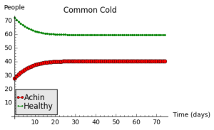
Click to go to the Sage applet for the common cold model.

We did not get to discuss this model in detail in class. An important thing to notice is that depending on the combination of get well parameter $g$ and contact rate $c$ , the number of people carrying the cold does not decrease to $0$ , as it did for the headache. It turns out that these final numbers (we call them the equilibrium), do not depend on the number of people who had the disease initially. Try it out! Let’s say that we use $A^\ast$ and $H^\ast$ for Achin’ and Healthy people at the end. Can you figure out how to calculate the values for $A^\ast$ and $H^\ast$ from the model equations? (Hint: If the number of sick does not change, this means that $A[t] = A^\ast$ and $A[t+1] = A^\ast$ , and similarly for $H^\ast$ ). You can see if your calculations are correct by clicking Show the equilibrium on the applet.

Finally, we briefly discussed the model for the spread of zombie disease. Instead of Healthy and Achin’, we counted the number of Humans, Zombies, and Dead, according to the following graph.

Compartment model of a zombie infection

Can you write out the equation for the model yourself? How would you modify the model to account for back ups sent to the city to ward off the zombies every day?

The model for zombie dynamics is more properly called the SIR model and it is probably the most famous compartmental model of them all. It captures well the dynamics of many infections, including mumps, measles, and rubella, all of which we now vaccinate against (What does vacca mean in Latin, and why is that word connected to immunizations?)

Click to go to the Sage applet for the zombie infection model.

Finally, I had a lot of fun talking about math with everybody at Madison Math Circle. Stay curious!

Madison Math Circle: Mathematics of epidemics

Leave a comment Cancel reply

Categories

Madison Math Circle: Mathematics of epidemics

Share this:

Leave a comment Cancel reply

Categories